Monte Carlo simulation runs thousands of random "what if" scenarios to show the range of possible outcomes for a portfolio. Instead of assuming a single fixed return, it draws from a spread of possible returns to produce a realistic picture of what could happen, along with the likelihood of each outcome.

This approach solves a basic problem with traditional projections: they assume your portfolio will grow at the same rate every year, which rarely happens in practice. A portfolio expected to average 7% annually will not return 7% in any single year. Monte Carlo captures this reality by treating each year's return as uncertain, producing a range of possible results rather than a single number.

Conceptual Framework

Monte Carlo simulation is a type of random sampling method. The core idea is straightforward: when a system has too many moving parts to predict exactly, you can run it many times with random inputs and look at the pattern of results. In portfolio analysis, the main moving part is the uncertain future return of each investment.

The method is named after the Monte Carlo Casino in Monaco. Physicists Stanislaw Ulam and John von Neumann coined the term during the Manhattan Project when they discovered that random sampling could solve math problems that were otherwise too complex to calculate directly. Financial applications followed in the 1960s and 1970s as computers became powerful enough to run thousands of simulations quickly.

Core Assumptions

Every Monte Carlo model makes assumptions about how investment returns behave. The most common assumptions, and their limitations, include:

• Return distribution: Most versions assume returns follow a bell curve (normal distribution), which underestimates the chance of extreme events. In reality, large market crashes and rallies happen more often than a bell curve predicts. More advanced models use "fat-tailed" distributions that better account for these extremes.
• Stable conditions: The model usually assumes that average returns, volatility (the size of price swings), and correlations between investments stay the same over the entire simulation period. In practice, markets shift between calm and turbulent periods, and these properties change along with them.
• Each period is independent: Basic versions assume that one month's return has no connection to the next. This ignores well-known patterns like momentum (winners keep winning), mean reversion (prices bouncing back), and volatility clustering (big moves tend to follow big moves).
• How investments move together: When simulating multiple investments, the model needs assumptions about how they relate to each other. In practice, investments tend to become more correlated during market stress, exactly when diversification matters most. Fixed assumptions about these relationships can understate risk.

Simulation Architecture

A Monte Carlo simulation for portfolio analysis follows a five-step process, from setting up the inputs to analyzing the range of results.

Parameter Estimation

The simulation starts with setting the inputs that describe how each investment behaves. At a minimum, you need an expected average return and a measure of how much returns vary (volatility). If simulating multiple investments together, you also need to specify how they relate to each other (their correlations).

A key decision is which historical period to base these inputs on. Longer time periods provide more data but may include conditions that are no longer relevant. Shorter periods capture recent conditions but are less reliable because the sample is smaller. There is no perfect answer; it requires judgment about which historical environment best represents the future.

Random Sampling and Path Generation

Each simulation trial generates a complete time series of returns by sampling from the specified distribution. For a 30-year retirement simulation with monthly returns, each trial produces 360 random draws. A typical simulation runs 10,000 trials, generating 3.6 million individual return observations.

When simulating multiple investments, the random draws need to reflect how those investments relate to each other. A mathematical technique called Cholesky decomposition transforms independent random numbers into correlated ones. This ensures that if stocks and bonds are assumed to move in opposite directions, the simulated paths maintain that relationship.

Outcome Aggregation

After generating thousands of return paths, the simulation applies the portfolio's cash flow rules (contributions, withdrawals, rebalancing) to each path and records the ending value. The collection of ending values forms an empirical probability distribution of outcomes. Key outputs include:

• Success probability: The percentage of trials where the portfolio survived the full time horizon without depletion. This is the most commonly cited output in retirement planning applications.
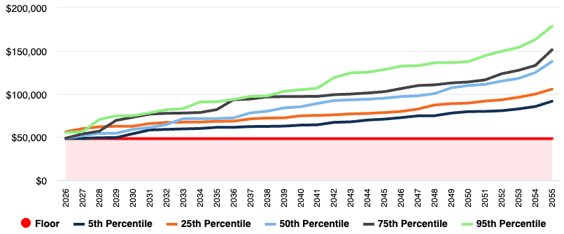
• Percentile outcomes: The 5th, 25th, 50th, 75th, and 95th percentile ending values, providing a range from pessimistic to optimistic scenarios.
• Shortfall magnitude: For trials that fail, the average shortfall amount and timing. A plan that fails at year 28 is meaningfully different from one that fails at year 15.

Risk Architecture

Monte Carlo simulation is a risk measurement tool, but it introduces its own risks that users should understand.

Model Risk

The biggest risk is that the assumptions built into the model do not match how markets actually behave. If the model assumes a bell-curve distribution but real markets produce more extreme events than a bell curve predicts, the simulation will undercount the chance of large losses. This matters most when the whole point of the simulation is to estimate the risk of extreme outcomes.

A second risk is that the inputs change depending on which historical period you look at. A simulation based on data from 2009 onward (mostly a rising market) will produce very different results than one based on the full 1926-to-present record. Neither is "right"; they reflect different views of what the future might look like.

Known Limitations

Practical Considerations

How Many Simulations?

More simulations produce more stable results, but at some point adding more does not meaningfully change the answer. For most financial applications, 10,000 trials are enough. If you need to estimate the risk of very rare, extreme events, you may need 50,000 or more trials to get reliable numbers.

Retirement Planning Applications

Monte Carlo simulation is widely used in retirement planning because the core question ("Will my money last 30 years?") has no simple formula. The answer depends on the interaction between unpredictable returns, inflation, and regular withdrawals. Critically, the order in which returns occur matters as much as their average: a big loss early in retirement is far more damaging than the same loss later.

Financial planning platforms like MaxiFi Planner use Monte Carlo simulations to project retirement outcomes. These tools generate percentile fan charts that let advisors and clients visualize how withdrawal strategies perform across thousands of simulated market environments rather than relying on a single deterministic forecast.

Common Extensions

More advanced versions of Monte Carlo simulation address some of the limitations described above:

• Regime-switching models: Let the simulation shift between "calm market" and "turbulent market" settings, so it can capture the reality that volatility and correlations between investments increase during downturns.
• Bootstrap simulation: Instead of assuming a mathematical distribution, this approach draws returns directly from actual historical data. This preserves the real shape of past returns, including extreme events, without needing to pick a specific distribution.
• Block bootstrap: Draws chunks of consecutive historical returns (e.g., a block of 12 months) rather than individual months. This preserves patterns like volatility clustering (big moves following big moves) that get lost when you shuffle individual months randomly.
• Mirror-image draws: A technique that generates each random scenario alongside its opposite. This makes the results converge faster, meaning you need fewer trials to get reliable answers.

Related Models

Further Reading

• Glasserman, P. (2003). Monte Carlo Methods in Financial Engineering. Springer (Stochastic Modelling and Applied Probability, Vol. 53).
• Jorion, P. (2007). Value at Risk: The New Benchmark for Managing Financial Risk. McGraw-Hill.
• Bengen, W.P. (1994). "Determining Withdrawal Rates Using Historical Data." Journal of Financial Planning.
• Pfau, W.D. (2013). "A Broader Framework for Determining an Efficient Frontier for Retirement Income." Journal of Financial Planning.
• Metropolis, N. and Ulam, S. (1949). "The Monte Carlo Method." Journal of the American Statistical Association, 44(247), 335–341.
• "Simulation Methods" (CFA Institute Professional Learning).
• "Using Monte Carlo Methods for Retirement Simulations" (arXiv, 2023).